7.8 Identifying errors in algorithms
Trace tables and carefully chosen test data do more than show what an algorithm does. They can expose errors, show exactly where a wrong result appears, and help you improve the algorithm so that it works for a wider range of inputs.
Using trace tables to find errors
The previous topic showed how a trace table records each variable whenever its value changes. The same technique can be used to identify and correct errors. You run the algorithm with suitable test data, compare the actual output with the expected result, and investigate any step that produces the wrong value.
The textbook revisits the algorithm that is intended to find the largest and smallest values from ten inputs. In its first version, the starting values are:
A ← 0
B ← 0
C ← 100
For the test data 400, 800, 190, 170, 300, 110, 600, 150, 130, 900, the trace table finishes with B = 900 and C = 100. B is correct, but C is wrong because the smallest input is 110.
| A | B | C | X | OUTPUT |
|---|---|---|---|---|
| 0 | 0 | 100 | ||
| 1 | 400 | 400 | ||
| 2 | 800 | 800 | ||
| 3 | 190 | |||
| 4 | 170 | |||
| 5 | 300 | |||
| 6 | 110 | |||
| 7 | 600 | |||
| 8 | 150 | |||
| 9 | 130 | |||
| 10 | 900 | 900 | ||
| 900 100 |
X < C is never true. C therefore never changes, even though 100 was not one of the input values.The same type of problem occurs with negative test data. If all ten values are negative, B begins at 0 and no negative input can satisfy X > B. The algorithm can therefore output 0 as the maximum even though 0 was never entered.
First improvement: use much wider starting limits
A simple improvement is to choose provisional values that are far outside the range expected in most test data. The textbook changes the starting values to B = -1,000,000 and C = 1,000,000.
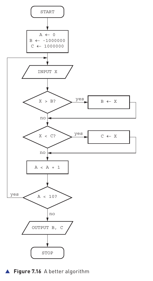
This version works for a much larger range of positive and negative numbers. A normal value is likely to be greater than -1,000,000, so B can be replaced by a real input. A normal value is also likely to be less than 1,000,000, so C can be replaced by a real input.
However, the algorithm is still not guaranteed to work for every possible set of numbers. If all values are less than -1,000,000, B could remain -1,000,000 even though that value was never entered. Likewise, if all values are greater than 1,000,000, C could remain 1,000,000.
A robust solution: initialise from the first input
To make the algorithm work for any set of numbers, the provisional maximum and minimum should come from the data itself. The standard method shown in the textbook is to input the first value and assign it to both B and C.
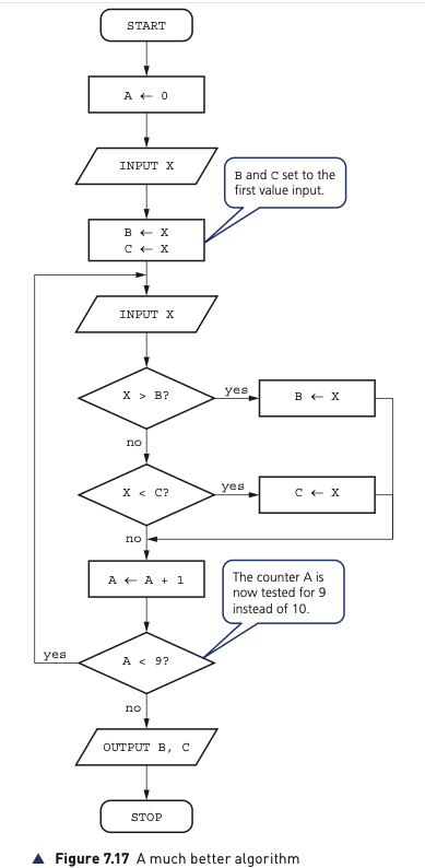
The improved sequence is:
A ← 0
INPUT X
B ← X
C ← X

REPEAT
  INPUT X
  IF X > B
    THEN
      B ← X
  ENDIF
  IF X < C
    THEN
      C ← X
  ENDIF
  A ← A + 1
UNTIL A = 9

OUTPUT B, C
The first input is already counted by being placed directly into B and C. The loop therefore processes only the remaining nine values, which is why the counter is tested against 9 rather than 10.
This removes the arbitrary starting limits. Whether the values are all positive, all negative, very large, very small or mixed, both provisional values begin as a genuine member of the input list.
Testing the corrected algorithm
The textbook supplies this test set for the corrected version:
-97, 12390, 0, 77, 359, -2, -89, 5000, 21, 67The correct maximum is 12390 and the correct minimum is -97. A dry run should confirm these values.
A reliable error-finding method
When an algorithm gives the wrong result, use a structured approach rather than guessing:
| Step | What to do |
|---|---|
| 1 | State what the algorithm is supposed to do. |
| 2 | Choose test data that can expose likely weaknesses, including unusual or extreme values. |
| 3 | Work through the algorithm exactly as written using a trace table. |
| 4 | Compare the actual output with the result you know should be produced. |
| 5 | Find the first point where the trace stops behaving as expected. |
| 6 | Change the algorithm to remove the cause of the error. |
| 7 | Dry run the amended algorithm again, using several suitable test sets. |
Topic 7.8 demonstrates why choice of test data matters. The original algorithm appeared to work with the earlier positive values between 0 and 100, but different data revealed that its initial values were unsafe assumptions.